Loading Tracking Data#
In this notebook, we will walk through the process of loading tracking data from different format into Megabouts.
Loading dependencies
import numpy as np
import matplotlib.pyplot as plt

from megabouts.tracking_data import (
    TrackingConfig,
    FullTrackingData,
    HeadTrackingData,
    TailTrackingData,
    load_example_data,
)
Tracking method and data format#
Megabouts handle a variety of tracking methods:
Full Tracking
Head Tracking
Tail Tracking
Different Input Formats: the tracking data can be loaded using two format, the
keypointorpostureformat.Units: position should be provided in mm and angle in radian.
TrackingData Class#
The class FullTrackingData,HeadTrackingData and TailTrackingData handles the input and reformats the movement data into a standardized format.
Tail Tracking Requirements#
At least 4 keypoints from the swim bladder to the tail tip are required to load tail tracking data.
The tail posture will be interpolated to 11 equidistant points.
Show code cell source
from IPython.display import SVG, display

display(SVG(filename="megabouts_tracking_configuration.svg"))

Loading Example Data#
The load_example_data function allows to load example .csv dataset corresponding to several tracking configuration (fulltracking_posture, SLEAP_fulltracking, HR_DLC, zebrabox_SLEAP). In the following sections we demonstrates how to import the example dataset into the TrackingData class.
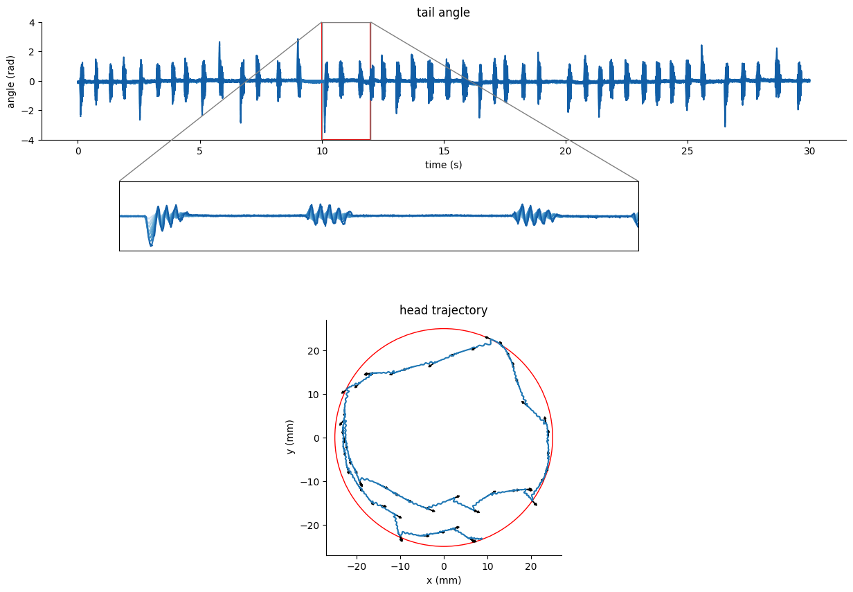
High-resolution tracking for freely-swimming zebrafish#
df_recording, fps, mm_per_unit = load_example_data("fulltracking_posture")
df_recording.head(5)
| head_x | head_y | head_angle | tail_angle_0 | tail_angle_1 | tail_angle_2 | tail_angle_3 | tail_angle_4 | tail_angle_5 | tail_angle_6 | tail_angle_7 | tail_angle_8 | tail_angle_9 | |
|---|---|---|---|---|---|---|---|---|---|---|---|---|---|
| 0 | -22.979468 | 3.989994 | -2.218813 | -0.101865 | -0.092813 | -0.107645 | -0.110575 | -0.047699 | -0.145887 | -0.130414 | -0.058892 | -0.128705 | NaN |
| 1 | -22.977063 | 3.998453 | -2.225990 | -0.082618 | -0.087957 | -0.096951 | -0.092459 | -0.119418 | -0.043354 | -0.099788 | -0.101741 | -0.171555 | NaN |
| 2 | -22.978636 | 3.993386 | -2.221900 | -0.093377 | -0.095235 | -0.094292 | -0.105936 | -0.073785 | -0.084193 | -0.144378 | -0.112398 | -0.042585 | NaN |
| 3 | -22.981788 | 3.992900 | -2.223969 | -0.092590 | -0.083650 | -0.100938 | -0.088223 | -0.097370 | -0.099559 | -0.101538 | -0.091272 | -0.021459 | NaN |
| 4 | -22.977184 | 3.999899 | -2.226333 | -0.086849 | -0.081982 | -0.096705 | -0.118475 | -0.046264 | -0.136459 | -0.115412 | -0.085300 | -0.015487 | NaN |
We first define the tracking configuration given the framerate and tracking method:
tracking_cfg = TrackingConfig(fps=fps, tracking="full_tracking")
We first extract the posture from the
df_recordingdataframe and convert position to mm
head_x = df_recording["head_x"].values * mm_per_unit
head_y = df_recording["head_y"].values * mm_per_unit
head_yaw = df_recording["head_angle"].values
tail_angle = df_recording.filter(like="tail_angle").values
Finally we input the postural array into the
FullTrackingDataclass:
tracking_data = FullTrackingData.from_posture(
    head_x=head_x, head_y=head_y, head_yaw=head_yaw, tail_angle=tail_angle
)
We can use the dataframe
tracking_data.tail_dfandtracking_data.traj_dfto visualize the tail and head trajectory
Show code cell source
from mpl_toolkits.axes_grid1.inset_locator import mark_inset
import matplotlib.patches as patches
from cycler import cycler

num_colors = 10
blue_cycler = cycler(color=plt.cm.Blues(np.linspace(0.2, 0.9, num_colors)))

# Generate time and data for plotting
t = np.arange(tracking_data.T) / tracking_cfg.fps
IdSt = 0  # np.random.randint(tracking_data.T)
Duration = 30 * tracking_cfg.fps
short_interval = slice(
    IdSt + 10 * tracking_cfg.fps, IdSt + 12 * tracking_cfg.fps
)  # 10-second interval

# Create figure and subplots
fig, ax = plt.subplots(3, 1, figsize=(15, 10), height_ratios=[0.5, 0.5, 1])

# Main plot for tail angle with zoom box (ax[0])
ax[0].set_prop_cycle(blue_cycler)
ax[0].plot(
    t[IdSt : IdSt + Duration], tracking_data.tail_df.iloc[IdSt : IdSt + Duration]
)
ax[0].set(
    **{
        "title": "tail angle",
        "xlabel": "time (s)",
        "ylabel": "angle (rad)",
        "ylim": (-4, 4),
    }
)
ax[0].add_patch(
    patches.Rectangle(
        (t[short_interval.start], -4),
        2,
        8,
        linewidth=1.5,
        edgecolor="red",
        facecolor="none",
    )
)

# Hide ax[1]
ax[1].axis("off")

# Trajectory plot with circle (ax[2])
ax[2].plot(
    tracking_data.traj_df.x.iloc[IdSt : IdSt + Duration],
    tracking_data.traj_df.y.iloc[IdSt : IdSt + Duration],
)
ax[2].add_artist(plt.Circle((0.0, 0.0), 25, color="red", fill=False))
ax[2].set(
    **{
        "xlim": (-27, 27),
        "ylim": (-27, 27),
        "title": "head trajectory",
        "aspect": "equal",
        "xlabel": "x (mm)",
        "ylabel": " y (mm)",
    }
)

# Inset axis for zoomed tail angle (above ax[1])
inset_ax = fig.add_axes([0.2, 0.55, 0.5, 0.1])
inset_ax.set_prop_cycle(blue_cycler)
inset_ax.plot(t[short_interval], tracking_data.tail_df.iloc[short_interval])
inset_ax.set(
    **{"xlim": (t[short_interval.start], t[short_interval.stop]), "ylim": (-4, 4)}
)
inset_ax.tick_params(
    which="both", bottom=False, left=False, labelbottom=False, labelleft=False
)
mark_inset(ax[0], inset_ax, loc1=1, loc2=2, fc="none", ec="0.5")
[axis.spines[["right", "top"]].set_visible(False) for axis in [ax[0], ax[2]]]
for i in range(IdSt, IdSt + Duration, 350):
    ax[2].arrow(
        tracking_data.traj_df["x"][i],
        tracking_data.traj_df["y"][i],
        np.cos(tracking_data.traj_df["yaw"][i]),
        np.sin(tracking_data.traj_df["yaw"][i]),
        head_width=0.5,
        head_length=0.5,
        fc="k",
        ec="k",
    )
[axis.spines[["right", "top"]].set_visible(False) for axis in [ax[0], ax[1]]]


plt.show()
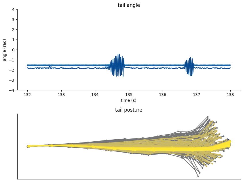
Tail tracking in head-restrained condition#
The following example correspond to tail tracking using DeepLabCut at 250fps.
df_recording, fps, mm_per_unit = load_example_data("HR_DLC")
df_recording = df_recording["DLC_resnet50_Zebrafish"]
df_recording.head(5)
| head_rostral | head_caudal | tail0 | tail1 | ... | tail7 | tail8 | tail9 | tail10 | |||||||||||||
|---|---|---|---|---|---|---|---|---|---|---|---|---|---|---|---|---|---|---|---|---|---|
| x | y | likelihood | x | y | likelihood | x | y | likelihood | x | ... | likelihood | x | y | likelihood | x | y | likelihood | x | y | likelihood | |
| 0 | 173.163055 | 2.995913 | 0.999985 | 177.695465 | 40.429813 | 0.999986 | 180.415710 | 80.903931 | 0.999986 | 180.984070 | ... | 0.999699 | 176.853455 | 255.031494 | 0.999377 | 177.243164 | 275.275574 | 0.999759 | 182.846207 | 295.142303 | 0.998607 |
| 1 | 172.605087 | 2.485497 | 0.999978 | 177.292572 | 40.164856 | 0.999983 | 180.129837 | 80.911896 | 0.999986 | 180.985275 | ... | 0.999701 | 176.757172 | 254.480911 | 0.999264 | 177.075943 | 274.513336 | 0.999753 | 181.680435 | 294.865326 | 0.998829 |
| 2 | 172.442398 | 2.889864 | 0.999985 | 176.992661 | 40.337017 | 0.999978 | 179.854385 | 81.170639 | 0.999989 | 180.823120 | ... | 0.999689 | 176.803375 | 254.154663 | 0.999175 | 177.024689 | 274.277985 | 0.999738 | 181.801056 | 294.448608 | 0.998983 |
| 3 | 173.055008 | 3.141099 | 0.999988 | 177.103790 | 40.811363 | 0.999983 | 179.919678 | 81.260208 | 0.999992 | 180.836472 | ... | 0.999672 | 176.752884 | 253.947128 | 0.999102 | 176.918564 | 274.054047 | 0.999732 | 181.057159 | 294.441162 | 0.999080 |
| 4 | 172.497513 | 3.288911 | 0.999988 | 176.927582 | 40.711155 | 0.999981 | 179.895370 | 81.267540 | 0.999990 | 180.830780 | ... | 0.999690 | 176.760941 | 254.114883 | 0.999147 | 176.989029 | 274.209351 | 0.999724 | 181.283981 | 294.534668 | 0.999020 |
5 rows × 39 columns
We first define the tracking configuration given the framerate and tracking method:
tracking_cfg = TrackingConfig(fps=fps, tracking="tail_tracking")
We will place NaN on the tail keypoints coordinates when the likelihood is below a threshold
kpts_list = [f"tail{i}" for i in range(11)]
thresh_score = 0.99
for kps in kpts_list:
    df_recording.loc[df_recording[(kps, "likelihood")] < thresh_score, (kps, "x")] = (
        np.nan
    )
    df_recording.loc[df_recording[(kps, "likelihood")] < thresh_score, (kps, "y")] = (
        np.nan
    )
We extract the tail keypoints coordinates and convert them in millimeters:
tail_x = df_recording.loc[
    :,
    [
        (segment, "x")
        for segment, coord in df_recording.columns
        if segment in kpts_list and coord == "x"
    ],
].values
tail_y = df_recording.loc[
    :,
    [
        (segment, "y")
        for segment, coord in df_recording.columns
        if segment in kpts_list and coord == "y"
    ],
].values

tail_x = tail_x * mm_per_unit
tail_y = tail_y * mm_per_unit
Finally we input the postural array into the
TailTrackingDataclass:
tracking_data = TailTrackingData.from_keypoints(tail_x=tail_x, tail_y=tail_y)
We can use the dataframe
tracking_data.tail_dfto visualize the tail angle
Show code cell source
t = np.arange(tracking_data.T) / tracking_cfg.fps
IdSt = 33000  # np.random.randint(tracking_data.T)
Duration = 6 * tracking_cfg.fps

fig, ax = plt.subplots(2, 1, figsize=(10, 8), height_ratios=[1, 1])
ax[0].set_prop_cycle(blue_cycler)
ax[0].plot(
    t[IdSt : IdSt + Duration], tracking_data.tail_df.iloc[IdSt : IdSt + Duration, :]
)
ax[0].set(title="tail angle", ylim=[-4, 4], xlabel="time (s)", ylabel="angle (rad)")

cmap = plt.get_cmap("cividis")
for i in range(IdSt, IdSt + Duration):
    ax[1].plot(
        tracking_data._tail_y[i, :],
        tracking_data._tail_x[i, :],
        ".-",
        color=cmap((i - IdSt) / Duration),
    )
ax[1].set(title="tail posture", aspect="equal")
ax[1].tick_params(
    which="both", bottom=False, left=False, labelbottom=False, labelleft=False
)
[axis.spines[["right", "top"]].set_visible(False) for axis in [ax[0], ax[1]]]

plt.show()
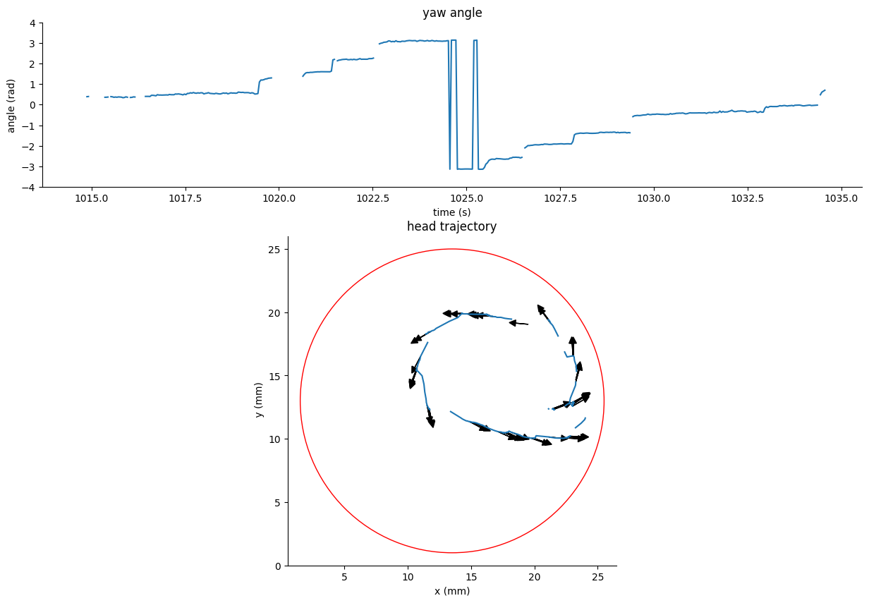
Low resolution centroid tracking from the Zebrabox config#
The following example correspond to head and swim-bladder tracking using SLEAP on video data from the Zebrabox system.
df_recording, fps, mm_per_unit = load_example_data("zebrabox_SLEAP")
df_recording.head(5)
| track | frame_idx | instance.score | swim_bladder.x | swim_bladder.y | swim_bladder.score | mid_eye.x | mid_eye.y | mid_eye.score | |
|---|---|---|---|---|---|---|---|---|---|
| 0 | NaN | 0 | 0.732962 | 111.594383 | 122.333862 | 0.834701 | 120.034706 | 118.537903 | 0.827217 |
| 1 | NaN | 1 | 0.733804 | 111.594688 | 122.324165 | 0.834202 | 120.029968 | 118.541588 | 0.826500 |
| 2 | NaN | 2 | 0.734254 | 111.595268 | 122.321350 | 0.834111 | 120.029823 | 118.539879 | 0.826383 |
| 3 | NaN | 3 | 0.732529 | 111.611320 | 122.310394 | 0.831942 | 120.030312 | 118.545074 | 0.827309 |
| 4 | NaN | 4 | 0.733020 | 111.588501 | 122.294258 | 0.832367 | 120.054565 | 118.565849 | 0.820087 |
We first define the tracking configuration given the framerate and tracking method:
tracking_cfg = TrackingConfig(fps=fps, tracking="head_tracking")
We will place NaN on the keypoints coordinates when the score is below a threshold
thresh_score = 0.75
is_tracking_bad = (df_recording["swim_bladder.score"] < thresh_score) | (
    df_recording["mid_eye.score"] < thresh_score
)
df_recording.loc[is_tracking_bad, "mid_eye.x"] = np.nan
df_recording.loc[is_tracking_bad, "mid_eye.y"] = np.nan
df_recording.loc[is_tracking_bad, "swim_bladder.x"] = np.nan
df_recording.loc[is_tracking_bad, "swim_bladder.y"] = np.nan
We extract the head and swim bladder keypoints coordinates and convert them in millimeters:
head_x = df_recording["mid_eye.x"].values * mm_per_unit
head_y = df_recording["mid_eye.y"].values * mm_per_unit
swimbladder_x = df_recording["swim_bladder.x"].values * mm_per_unit
swimbladder_y = df_recording["swim_bladder.y"].values * mm_per_unit
Finally we input the keypoints into the
HeadTrackingDataclass:
tracking_data = HeadTrackingData.from_keypoints(
    head_x=head_x,
    head_y=head_y,
    swimbladder_x=swimbladder_x,
    swimbladder_y=swimbladder_y,
)
We can use the dataframe
tracking_data.traj_dfto visualize the head position and yaw
Show code cell source
from mpl_toolkits.axes_grid1.inset_locator import mark_inset
import matplotlib.patches as patches

num_colors = 10
blue_cycler = cycler(color=plt.cm.Blues(np.linspace(0.2, 0.9, num_colors)))

# Generate time and data for plotting
t = np.arange(tracking_data.T) / tracking_cfg.fps
IdSt = 25365  # np.random.randint(tracking_data.T)
Duration = 20 * tracking_cfg.fps
short_interval = slice(
    IdSt + 10 * tracking_cfg.fps, IdSt + 12 * tracking_cfg.fps
)  # 10-second interval

# Create figure and subplots
fig, ax = plt.subplots(2, 1, figsize=(15, 10), height_ratios=[0.5, 1])

# Main plot for tail angle with zoom box (ax[0])
ax[0].plot(
    t[IdSt : IdSt + Duration], tracking_data.traj_df["yaw"].iloc[IdSt : IdSt + Duration]
)
ax[0].set(
    **{
        "title": "yaw angle",
        "xlabel": "time (s)",
        "ylabel": "angle (rad)",
        "ylim": (-4, 4),
    }
)

# Trajectory plot with circle (ax[2])
ax[1].plot(
    tracking_data.traj_df.x.iloc[IdSt : IdSt + Duration],
    tracking_data.traj_df.y.iloc[IdSt : IdSt + Duration],
)
ax[1].add_artist(plt.Circle((13.5, 13), 12, color="red", fill=False))
ax[1].set(
    **{
        "xlim": (0.5, 26.5),
        "ylim": (0.0, 26.0),
        "title": "head trajectory",
        "aspect": "equal",
        "xlabel": "x (mm)",
        "ylabel": " y (mm)",
    }
)
for i in range(IdSt, IdSt + Duration, 10):
    ax[1].arrow(
        tracking_data.traj_df["x"][i],
        tracking_data.traj_df["y"][i],
        np.cos(tracking_data.traj_df["yaw"][i]),
        np.sin(tracking_data.traj_df["yaw"][i]),
        head_width=0.5,
        head_length=0.5,
        fc="k",
        ec="k",
    )
[axis.spines[["right", "top"]].set_visible(False) for axis in [ax[0], ax[1]]]

plt.show()
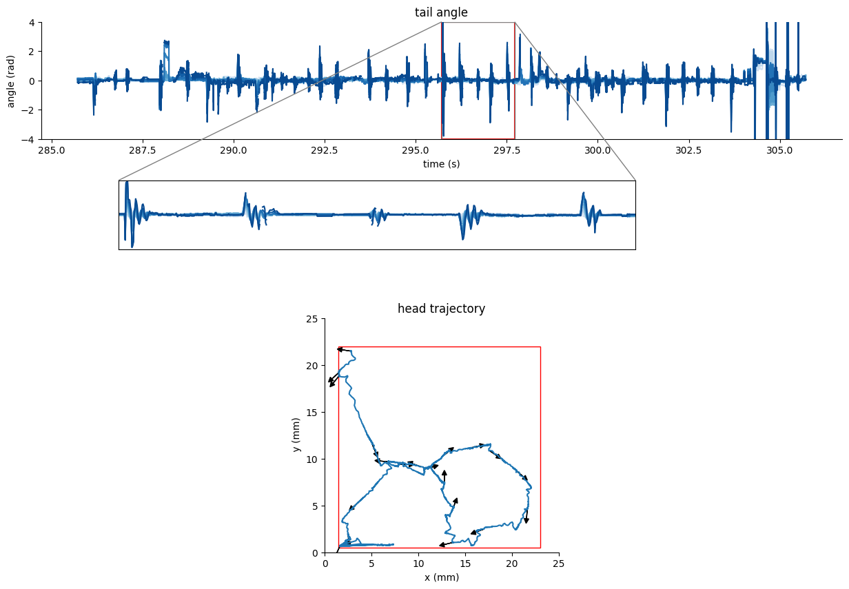
Noisy tracking of freely-swimming zebrafish#
The following example correspond to full tracking at 350fps. The fish posture is tracked using SLEAP but the keypoints are not reliably placed due to insufficient labelling.
df_recording, fps, mm_per_unit = load_example_data("SLEAP_fulltracking")
df_recording.head(5)
| track | frame_idx | instance.score | left_eye.x | left_eye.y | left_eye.score | right_eye.x | right_eye.y | right_eye.score | tail0.x | ... | tail1.score | tail2.x | tail2.y | tail2.score | tail3.x | tail3.y | tail3.score | tail4.x | tail4.y | tail4.score | |
|---|---|---|---|---|---|---|---|---|---|---|---|---|---|---|---|---|---|---|---|---|---|
| 0 | NaN | 0 | 0.977651 | 822.667358 | 839.635101 | 0.988699 | 807.832947 | 840.091492 | 0.953313 | 813.303932 | ... | 0.987229 | 807.466705 | 767.853134 | 1.027914 | 806.901657 | 747.167450 | 0.941431 | 803.414474 | 730.643631 | 0.821148 |
| 1 | NaN | 1 | 0.977400 | 822.669495 | 839.644699 | 0.988768 | 807.837723 | 840.099838 | 0.951950 | 813.305016 | ... | 0.987644 | 807.468445 | 767.856720 | 1.027526 | 806.901627 | 747.176315 | 0.941242 | 803.420502 | 730.653046 | 0.822505 |
| 2 | NaN | 2 | 0.977176 | 822.668884 | 839.653854 | 0.988344 | 807.838104 | 840.107727 | 0.950716 | 813.306580 | ... | 0.987669 | 807.469040 | 767.860291 | 1.027348 | 806.905151 | 747.177567 | 0.941105 | 803.416382 | 730.654694 | 0.820525 |
| 3 | NaN | 3 | 0.976941 | 822.670547 | 839.665436 | 0.989196 | 810.813538 | 840.147018 | 0.950221 | 813.307747 | ... | 0.988717 | 807.468109 | 767.858276 | 1.026542 | 806.905106 | 747.178329 | 0.940126 | 803.417862 | 730.658585 | 0.820215 |
| 4 | NaN | 4 | 0.976689 | 822.674286 | 839.674667 | 0.989967 | 810.819382 | 840.155060 | 0.949718 | 813.308144 | ... | 0.989073 | 807.468567 | 767.867950 | 1.026512 | 806.904449 | 747.200958 | 0.940060 | 803.418640 | 730.675385 | 0.824549 |
5 rows × 24 columns
We first define the tracking configuration given the framerate and tracking method:
tracking_cfg = TrackingConfig(fps=fps, tracking="full_tracking")
We will place NaN on the keypoints coordinates when the score is below a threshold
# Place nan where the score is below a threshold:
thresh_score = 0.0
for kps in ["left_eye", "right_eye", "tail0", "tail1", "tail2", "tail3", "tail4"]:
    df_recording.loc[df_recording["instance.score"] < thresh_score, kps + ".x"] = np.nan
    df_recording.loc[df_recording["instance.score"] < thresh_score, kps + ".y"] = np.nan
    df_recording.loc[df_recording[kps + ".score"] < thresh_score, kps + ".x"] = np.nan
    df_recording.loc[df_recording[kps + ".score"] < thresh_score, kps + ".y"] = np.nan
We extract the head and tail keypoints coordinates and convert them in millimeters:
head_x = (df_recording["left_eye.x"].values + df_recording["right_eye.x"].values) / 2
head_y = (df_recording["left_eye.y"].values + df_recording["right_eye.y"].values) / 2

tail_x = df_recording[["tail0.x", "tail1.x", "tail2.x", "tail3.x", "tail4.x"]].values
tail_y = df_recording[["tail0.y", "tail1.y", "tail2.y", "tail3.y", "tail4.y"]].values

head_x = head_x * mm_per_unit
head_y = head_y * mm_per_unit
tail_x = tail_x * mm_per_unit
tail_y = tail_y * mm_per_unit
Finally the keypoints arrays are loaded into the
FullTrackingDataclass:
tracking_data = FullTrackingData.from_keypoints(
    head_x=head_x, head_y=head_y, tail_x=tail_x, tail_y=tail_y
)
We can use the dataframe
tracking_data.tail_dfandtracking_data.traj_dfto visualize the fish posture.
Show code cell source
from mpl_toolkits.axes_grid1.inset_locator import mark_inset
import matplotlib.patches as patches

num_colors = 10
blue_cycler = cycler(color=plt.cm.Blues(np.linspace(0.2, 0.9, num_colors)))

# Generate time and data for plotting
t = np.arange(tracking_data.T) / tracking_cfg.fps
IdSt = 100000  # np.random.randint(tracking_data.T)
Duration = 20 * tracking_cfg.fps
short_interval = slice(
    IdSt + 10 * tracking_cfg.fps, IdSt + 12 * tracking_cfg.fps
)  # 10-second interval

# Create figure and subplots
fig, ax = plt.subplots(3, 1, figsize=(15, 10), height_ratios=[0.5, 0.5, 1])

# Main plot for tail angle with zoom box (ax[0])
ax[0].set_prop_cycle(blue_cycler)
ax[0].plot(
    t[IdSt : IdSt + Duration], tracking_data.tail_df.iloc[IdSt : IdSt + Duration]
)
ax[0].set(
    **{
        "title": "tail angle",
        "xlabel": "time (s)",
        "ylabel": "angle (rad)",
        "ylim": (-4, 4),
    }
)
ax[0].add_patch(
    patches.Rectangle(
        (t[short_interval.start], -4),
        2,
        8,
        linewidth=1.5,
        edgecolor="red",
        facecolor="none",
    )
)

# Hide ax[1]
ax[1].axis("off")

# Trajectory plot with circle (ax[2])
ax[2].plot(
    tracking_data.traj_df.x.iloc[IdSt : IdSt + Duration],
    tracking_data.traj_df.y.iloc[IdSt : IdSt + Duration],
)
ax[2].add_artist(plt.Rectangle((1.5, 0.5), 21.5, 21.5, color="red", fill=False))
ax[2].set(
    **{
        "xlim": (0, 25),
        "ylim": (0, 25),
        "title": "head trajectory",
        "aspect": "equal",
        "xlabel": "x (mm)",
        "ylabel": " y (mm)",
    }
)

# Inset axis for zoomed tail angle (above ax[1])
inset_ax = fig.add_axes([0.2, 0.55, 0.5, 0.1])
inset_ax.set_prop_cycle(blue_cycler)
inset_ax.plot(t[short_interval], tracking_data.tail_df.iloc[short_interval])
inset_ax.set(
    **{"xlim": (t[short_interval.start], t[short_interval.stop]), "ylim": (-4, 4)}
)
inset_ax.tick_params(
    which="both", bottom=False, left=False, labelbottom=False, labelleft=False
)
mark_inset(ax[0], inset_ax, loc1=1, loc2=2, fc="none", ec="0.5")
[axis.spines[["right", "top"]].set_visible(False) for axis in [ax[0], ax[2]]]
for i in range(IdSt, IdSt + Duration, 350):
    ax[2].arrow(
        tracking_data.traj_df["x"][i],
        tracking_data.traj_df["y"][i],
        np.cos(tracking_data.traj_df["yaw"][i]),
        np.sin(tracking_data.traj_df["yaw"][i]),
        head_width=0.5,
        head_length=0.5,
        fc="k",
        ec="k",
    )
[axis.spines[["right", "top"]].set_visible(False) for axis in [ax[0], ax[1]]]


plt.show()