Head-restrained pipeline

The following notebook illustrate the HeadRestrainedPipeline class.

• Several preprocessing steps are used for head-restrained recording of the tail angle:

  • Preprocessing of the tail angle. In contrast with freely-swimming, more emphasis should be put on adjusting the baseline substraction.

  • Sparse coding of the tail angle.

  • Computation of the tail vigor associated to each atom of the sparse coding.

• Loading dependencies

import numpy as np
import matplotlib.pyplot as plt
import matplotlib.gridspec as gridspec
from cycler import cycler

from megabouts.tracking_data import TrackingConfig, TailTrackingData, load_example_data
from megabouts.pipeline import HeadRestrainedPipeline

• Loading tracking data

df_recording, fps, mm_per_unit = load_example_data("HR_DLC")
df_recording = df_recording["DLC_resnet50_Zebrafish"]

tracking_cfg = TrackingConfig(fps=fps, tracking="tail_tracking")
kpts_list = [f"tail{i}" for i in range(11)]
thresh_score = 0.99
for kps in kpts_list:
    df_recording.loc[df_recording[(kps, "likelihood")] < thresh_score, (kps, "x")] = (
        np.nan
    )
    df_recording.loc[df_recording[(kps, "likelihood")] < thresh_score, (kps, "y")] = (
        np.nan
    )
tail_x = df_recording.loc[
    :,
    [
        (segment, "x")
        for segment, coord in df_recording.columns
        if segment in kpts_list and coord == "x"
    ],
].values
tail_y = df_recording.loc[
    :,
    [
        (segment, "y")
        for segment, coord in df_recording.columns
        if segment in kpts_list and coord == "y"
    ],
].values

tail_x = tail_x * mm_per_unit
tail_y = tail_y * mm_per_unit

tracking_data = TailTrackingData.from_keypoints(tail_x=tail_x, tail_y=tail_y)

• Defining the pipeline

pipeline = HeadRestrainedPipeline(tracking_cfg)

• In contrast with freely-swimming where the default baseline method is "median", the default baseline method for head-restrained pipeline is set to "whittaker".

pipeline.tail_preprocessing_cfg.baseline_method

'whittaker'

• Baseline Computation in Sparse Coding

Sparse coding is designed to capture high-frequency components in the signal. To handle low-frequency components effectively:

1. We first compute and subtract a baseline

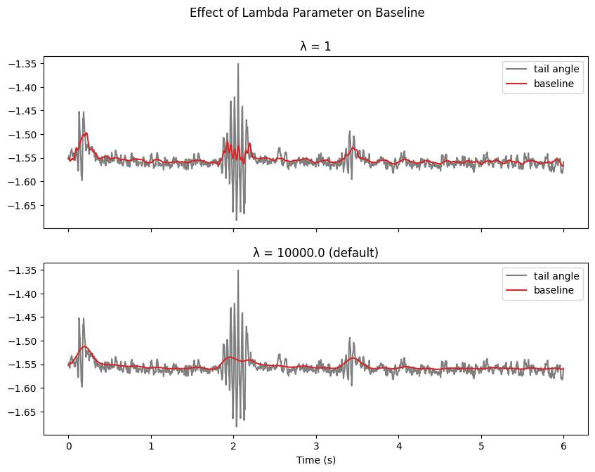
2. The baseline smoothness is controlled by λ (lambda parameter):

   • Higher λ values → smoother baseline

   • Lower λ values → baseline follows signal more closely

Show code cell source Hide code cell source

t = np.arange(tracking_data.T) / tracking_cfg.fps
IdSt = 20612
Duration = 1500
t_win = t[IdSt : IdSt + Duration] - t[IdSt]

fig, ax = plt.subplots(2, 1, figsize=(10, 7), sharex=True)
fig.suptitle("Effect of Lambda Parameter on Baseline")

for i, lmbda in enumerate([1, 1e4]):
    pipeline.tail_preprocessing_cfg.baseline_params["lmbda"] = lmbda
    tail = pipeline.preprocess_tail(tracking_data.tail_df)
    ax[i].plot(
        t_win, tail.angle[IdSt : IdSt + Duration, 7], "tab:gray", label="tail angle"
    )
    ax[i].plot(
        t_win,
        tail.angle_baseline[IdSt : IdSt + Duration, 7],
        "tab:red",
        label="baseline",
    )
    str_ = f"λ = {lmbda}"
    if lmbda == 1e4:
        str_ += " (default)"
    ax[i].set_title(str_)

    ax[i].legend()

ax[-1].set_xlabel("Time (s)")
plt.show()

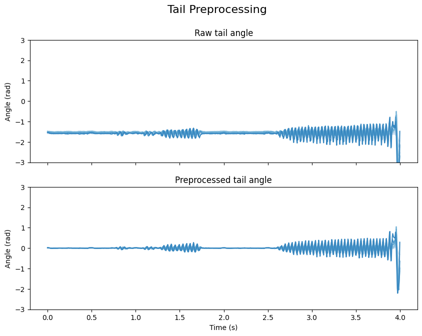
• Once the baseline is computed, it is substracted from the tail angle.

Show code cell source Hide code cell source

blue_cycler = cycler(color=plt.cm.Blues(np.linspace(0.2, 0.9, 10)))

t = np.arange(tracking_data.T) / tracking_cfg.fps
IdSt = 36000  # np.random.randint(tracking_data.T)
Duration = 1000
t_win = t[IdSt : IdSt + Duration] - t[IdSt]

# Prepare the data, titles, and subtitles
angle_data = [tail.angle, tail.angle_smooth]
subtitles = ["Raw tail angle", "Preprocessed tail angle"]

# Create subplots
fig, ax = plt.subplots(2, 1, figsize=(10, 7), sharex=True)

# Set a main title for the figure
fig.suptitle("Tail Preprocessing", fontsize=16)

# Loop over the axes, data, and subtitles
for axis, data, subtitle in zip(ax, angle_data, subtitles):
    axis.set_prop_cycle(blue_cycler)
    axis.plot(t_win, data[IdSt : IdSt + Duration, :7])
    axis.set(ylabel="Angle (rad)", ylim=(-3, 3))
    axis.set_title(subtitle, fontsize=12)

ax[-1].set_xlabel("Time (s)")
plt.show()

• Finally, sparse coding is applied to the preprocessed tail angle.

pipeline.sparse_coding_cfg

SparseCodingConfig(fps=250, lmbda=0.01, gamma=0.01, mu=0.05, window_inhib_ms=85, dict_peak_ms=28, vigor_win_ms=30)

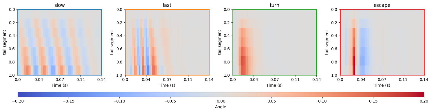
• Here is the dictionary of atoms used for sparse coding:

# Plot dictionary atoms
Dict = pipeline.sparse_coding_cfg.Dict

fig1 = plt.figure(figsize=(15, 4))
G = gridspec.GridSpec(2, 4, height_ratios=[4, 0.3])

atom_names = ["slow", "fast", "turn", "escape"]
colors = ["tab:blue", "tab:orange", "tab:green", "tab:red"]
for i in range(Dict.shape[-1]):
    ax = plt.subplot(G[0, i])
    im = ax.imshow(
        Dict[:, :, i].T,
        aspect="auto",
        vmin=-0.2,
        vmax=0.2,
        cmap="coolwarm",
        extent=[0, 100, 1, 0],
    )
    ax.set_ylabel("tail segment")
    ax.set_xticks(np.linspace(0, 100, 5))
    ax.set_xticklabels(np.round(np.linspace(0, 100 / 700, 5), 2))

    for spine in ax.spines.values():
        spine.set_edgecolor(colors[i])
        spine.set_linewidth(2)
    ax.set_xlabel("Time (s)")
    ax.set_title(atom_names[i])

cbar_ax = plt.subplot(G[1, :])
cbar = plt.colorbar(im, cax=cbar_ax, orientation="horizontal")
cbar.set_label("Angle")
plt.tight_layout()
plt.show()

• Running the sparse coding:

sparse_coding_result = pipeline.compute_sparse_coding(tail.angle_smooth)

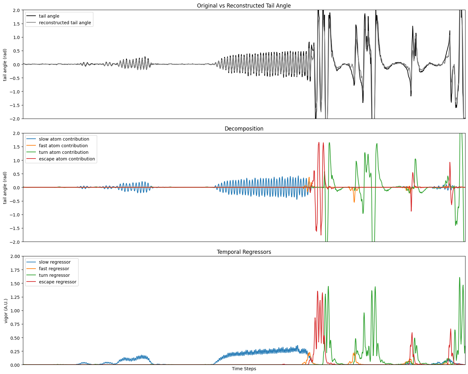
• We can now plot the results of the sparse coding. The color code of the atoms is the same as in the dictionary plot above.

Show code cell source Hide code cell source

fig, (ax1, ax2, ax3) = plt.subplots(3, 1, figsize=(15, 12), sharex=True)

t = np.linspace(0, Duration / 700, Duration)
IdSt, Duration = 36000, 1500
IdEd = IdSt + Duration
lim_ampl = 2

ax1.plot(
    sparse_coding_result.tail_angle[IdSt : IdSt + Duration, 6],
    color="k",
    label="tail angle",
)
ax1.plot(
    sparse_coding_result.tail_angle_hat[IdSt : IdSt + Duration, 6],
    color="tab:gray",
    label="reconstructed tail angle",
)
ax1.set_ylim(-lim_ampl, lim_ampl)
ax1.get_xaxis().set_ticks([])
ax1.set_title("Original vs Reconstructed Tail Angle")
ax1.set_ylabel("tail angle (rad)")
ax1.legend()

ax2.plot(
    sparse_coding_result.decomposition[IdSt : IdSt + Duration, :],
    label=[f"{name} atom contribution" for name in atom_names],
)
ax2.set_ylim(-lim_ampl, lim_ampl)
ax2.get_xaxis().set_ticks([])
ax2.set_title("Decomposition")
ax2.set_ylabel("tail angle (rad)")
ax2.legend()

ax3.plot(
    sparse_coding_result.regressor[IdSt : IdSt + Duration, :],
    label=[f"{name} regressor" for name in atom_names],
)
ax3.set_ylim(0, 2)
ax3.set_xlim(0, Duration)
ax3.set_title("Temporal Regressors")
ax3.set_xlabel("Time Steps")
ax3.set_ylabel("vigor (A.U.)")
ax3.legend()

plt.tight_layout()
plt.show()