Trajectory Preprocessing

The following notebook illustrate the TrajPreprocessing class how to run the preprocessing steps.

• Several preprocessing steps are available for the tail angle:

  • Interpolating missing values

  • Apply 1€ filter

• The kinematic vigor is also computed from the speed and will also be useful for segmentation into bouts:

• Loading dependencies

import numpy as np
import matplotlib.pyplot as plt

from megabouts.tracking_data import TrackingConfig, FullTrackingData, load_example_data
from megabouts.config import TrajPreprocessingConfig
from megabouts.preprocessing import TrajPreprocessing

Loading Data

• TrackingConfig and TrackingData similar to tutorial_Loading_Data

# Load data and set tracking configuration
df_recording, fps, mm_per_unit = load_example_data("SLEAP_fulltracking")
tracking_cfg = TrackingConfig(fps=fps, tracking="full_tracking")

# List of keypoints
keypoints = ["left_eye", "right_eye", "tail0", "tail1", "tail2", "tail3", "tail4"]

# Place NaN where the score is below a threshold
thresh_score = 0.0
for kps in keypoints:
    score_below_thresh = df_recording["instance.score"] < thresh_score
    df_recording.loc[
        score_below_thresh | (df_recording[f"{kps}.score"] < thresh_score),
        [f"{kps}.x", f"{kps}.y"],
    ] = np.nan

# Compute head and tail coordinates and convert to mm
head_x = ((df_recording["left_eye.x"] + df_recording["right_eye.x"]) / 2) * mm_per_unit
head_y = ((df_recording["left_eye.y"] + df_recording["right_eye.y"]) / 2) * mm_per_unit
tail_x = df_recording[[f"tail{i}.x" for i in range(5)]].values * mm_per_unit
tail_y = df_recording[[f"tail{i}.y" for i in range(5)]].values * mm_per_unit

# Create FullTrackingData object
tracking_data = FullTrackingData.from_keypoints(
    head_x=head_x.values, head_y=head_y.values, tail_x=tail_x, tail_y=tail_y
)

Run Preprocessing

• Define preprocessing config

traj_preprocessing_cfg = TrajPreprocessingConfig(fps=tracking_cfg.fps)

• Apply the trajectory preprocessing

traj_df_input = tracking_data.traj_df
traj = TrajPreprocessing(traj_preprocessing_cfg).preprocess_traj_df(traj_df_input)

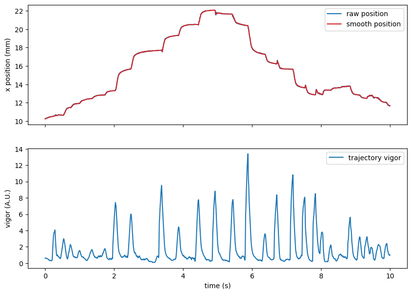
• traj.df contains information about the trajectory, the smooth values as well as the kinematic vigor:

traj.df.head(5)

	x	y	yaw	x_smooth	y_smooth	yaw_smooth	axial_speed	lateral_speed	yaw_speed	vigor	no_tracking
0	20.381254	20.996582	1.491111	20.381254	20.996582	1.491111	NaN	NaN	NaN	0.0	0.0
1	20.381340	20.996807	1.491013	20.381277	20.996642	1.491085	NaN	NaN	NaN	0.0	0.0
2	20.381337	20.997020	1.491086	20.381293	20.996742	1.491085	NaN	NaN	NaN	0.0	0.0
3	20.418551	20.997656	1.430916	20.391138	20.996983	1.475189	NaN	NaN	NaN	0.0	0.0
4	20.418671	20.997872	1.430749	20.399294	20.997219	1.461210	0.293531	-1.616157	-2.659344	0.0	0.0

• We can visualize the result of preprocessing:

Show code cell source Hide code cell source

t = np.arange(tracking_data.T) / tracking_cfg.fps
IdSt = np.random.randint(tracking_data.T)
Duration = 10 * tracking_cfg.fps
t_win = t[IdSt : IdSt + Duration] - t[IdSt]

fig, ax = plt.subplots(2, 1, figsize=(10, 7), sharex=True)
ax[0].plot(t_win, traj.x[IdSt : IdSt + Duration], label="raw position")
ax[0].plot(
    t_win,
    traj.x_smooth[IdSt : IdSt + Duration],
    label="smooth position",
    color="tab:red",
)
ax[1].plot(t_win, traj.vigor[IdSt : IdSt + Duration], label="trajectory vigor")
ax[0].set(ylabel="x position (mm)")
ax[1].set(ylabel="vigor (A.U.)")
ax[1].set(xlabel="time (s)")

for i in range(2):
    ax[i].legend()
plt.show()

Tuning 1€ filter

📝 There are two configurable parameters in the filter, the minimum cutoff frequency freq_cutoff_min and the speed coefficient beta.
Decreasing the minimum cutoff frequency decreases slow speed jitter. Increasing the speed coefficient decreases speed lag.
The parameters are set using two-step procedure:

Step 1

beta is set to 0 and freq_cutoff_min to 10Hz. Focus on a part of the recording where the fish is not swimming or swimming at low speed.
freq_cutoff_min is adjusted to remove jitter and preserve an acceptable lag during these slow movements.

traj_preprocessing_cfg = TrajPreprocessingConfig(
    fps=tracking_cfg.fps, freq_cutoff_min=10, beta=0
)

Show code cell source Hide code cell source

IdSt = 26800
Duration = 2 * tracking_cfg.fps
t_win = t[IdSt : IdSt + Duration] - t[IdSt]

x = traj_df_input.x
traj = TrajPreprocessing(traj_preprocessing_cfg).preprocess_traj_df(traj_df_input)
x_smooth = traj.df.x_smooth

fig, ax = plt.subplots(1, 1, figsize=(15, 4), sharex=True)
ax.set_title("Tuning " + r"$\text{freq_cutoff_min}$" + " during slow movement")
ax.plot(t_win, x[IdSt : IdSt + Duration], label="raw position")
ax.plot(
    t_win, x_smooth[IdSt : IdSt + Duration], label="smoothed position", color="tab:red"
)
ax.set(xlabel="time (s)", ylabel="x position (mm)")
ax.legend()
plt.show()

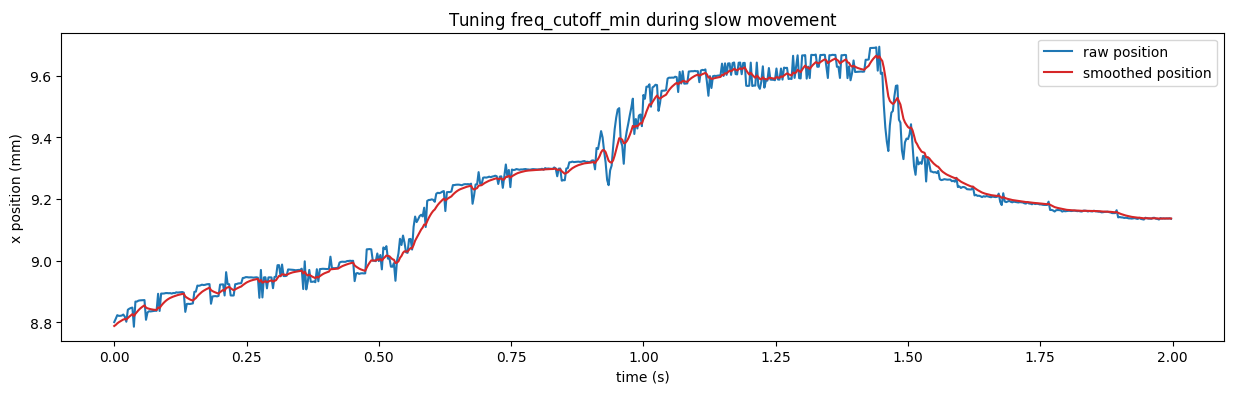
✅ Here a value close to 10Hz for freq_cutoff_min allows to smooth while keeping an acceptable lag

Step 2

Focus on a part of the recording where the fish is moving fast. Adjust beta with a focus on minimizing lag.

traj_preprocessing_cfg = TrajPreprocessingConfig(
    fps=tracking_cfg.fps, freq_cutoff_min=10, beta=1.4
)

Show code cell source Hide code cell source

IdSt = 81600  # np.random.randint(x.shape[0])
Duration = 2 * tracking_cfg.fps
t_win = t[IdSt : IdSt + Duration] - t[IdSt]

x = traj_df_input.x
traj = TrajPreprocessing(traj_preprocessing_cfg).preprocess_traj_df(traj_df_input)
x_smooth = traj.df.x_smooth

fig, ax = plt.subplots(1, 1, figsize=(15, 4), sharex=True)
ax.set_title("Tuning " + r"$\text{beta}$" + " during fast movement")
ax.plot(t_win, x[IdSt : IdSt + Duration], label="raw position")
ax.plot(
    t_win, x_smooth[IdSt : IdSt + Duration], label="smoothed position", color="tab:red"
)
ax.set(xlabel="time (s)", ylabel="x position (mm)")
ax.legend()
plt.show()

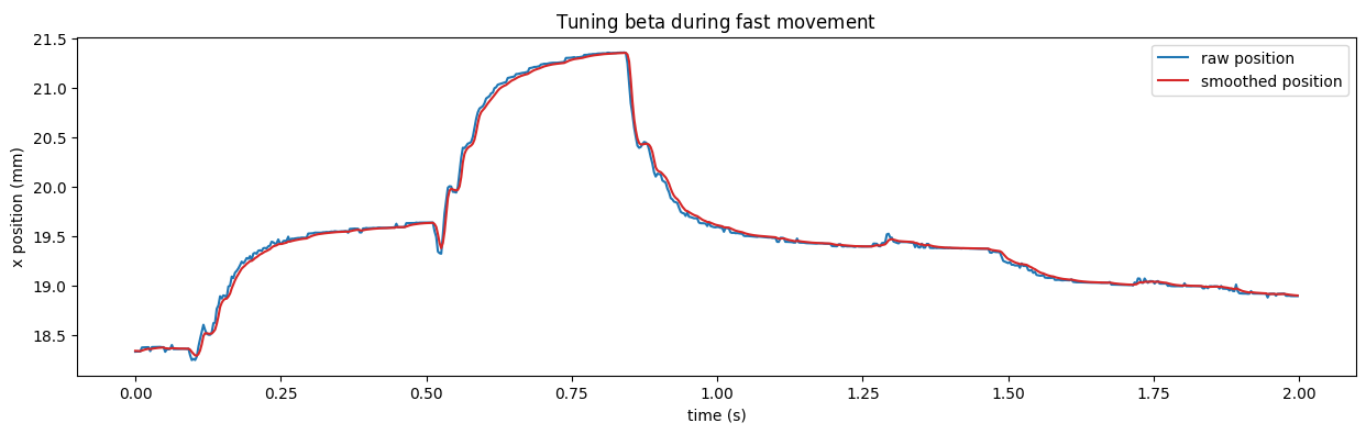
✅ Here we selected beta=1.4

📝 Note

Smoothing the trajectory data is optional for classifying tail bouts. The transformer model was trained on raw tracking data, so it can handle unsmoothed input just as well.